Insertion Sort
Insertion sort is an algorithm that attempts to solve the sorting problem. The sorting problem can be described as:
Input: A sequence of n numbers "a1, a2, ... , an".
Output: A permutation (reordering) "a'1, a'2, ... , a'n" of the input sequence such that a'1 <= a'2 <= ... <= a'n.
keys = Numbers that we wish to sort.
The input is received in the form of an array with n elements.
Insertion sort is an efficient algorithm to sort a small number of elements. Insertion sort works the way many people sort a hand of playing cards. We start with an empty left hand, and the cards face down on the table. We pick a card from the table and insert it into the correct position in the left hand. To find the correct position of the card in the left hand, we compare it with every card already in the hand, from right to left. At all times, the cards in the left hand are sorted.
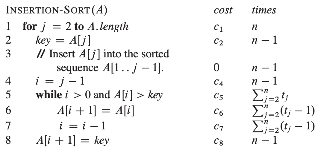
The pseudocode for the algorithm is given by INSERTION-SORT(A), where A is the input array, and A.length denotes the length of the array - n. The algorithm sorts the input numbers in place: it rearranges the numbers within the array A, with at most a constant number of elements stored outside the array at a time. So, the input is overwritten by the output as the algorithm executes.
INSERTION-SORT(A)
1. for j = 2 to A.length
2.     key = A[j]
3.     // Insert A[j] into the sorted sequence A[1 .. j - 1]/
4.     i = j - 1
5.     while i > 0 and A[i] > key
6.         A[i + 1] = A[i]
7.         i = i - 1
8.     A[i + 1] = key
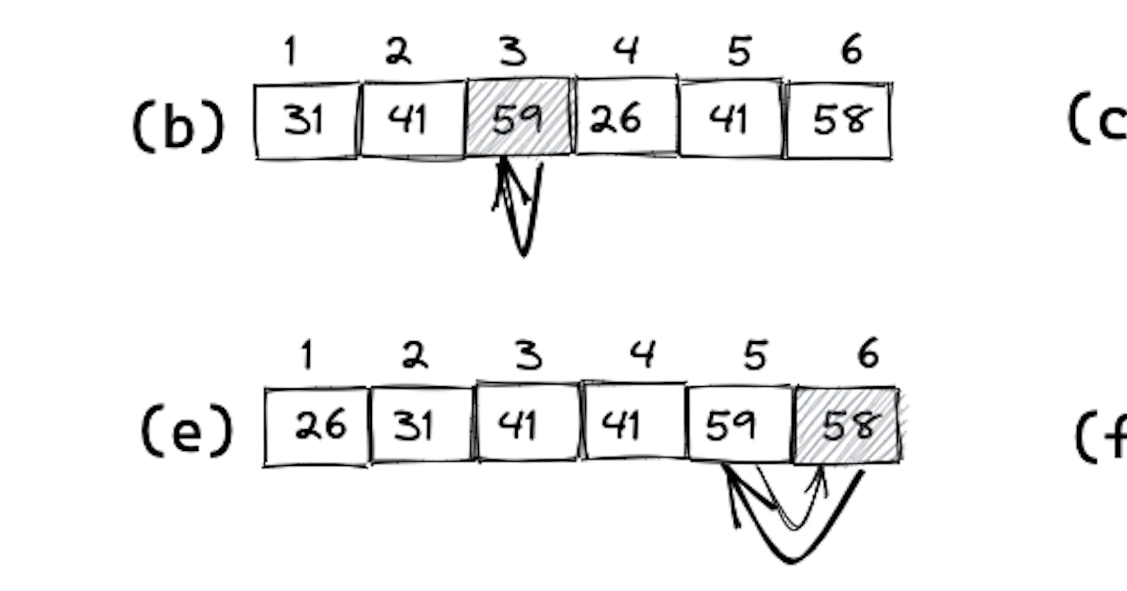
The operation of INSERTION-SORT on the array A = (31, 41, 59, 26, 41, 58) is displayed in the following figure. In the iterations of the for loop, the shaded rectangle holds the key taken from A[j] in line 2, which is compared with the values in rectangles to its left in the test of line 5. The rectangles are then moved inside the while loop to the right in line 6. (f) shows the final sorted array.

Loop invariants and the correctness of insertion sort
The index j indicates the "current card" being inserted in the hand. At the beginning of each iteration of the for loop, which is indexed by j, the subarray consisting of elements A[1 ... j - 1] constitutes the currently sorted hand, and the subarray A[j + 1 ... n] corresponds to the pile of cards still on the table. In fact, elements A[1 ... j - 1] are the elements originally in positions 1 through j - 1, but now in sorted order. We state these properties of A[1 ... j - 1] formally as a loop invariant:
At the start of each iteration of the for loop of lines 1–8, the subarray A[1 ... j - 1] consists of the elements originally in A[1 ... j - 1], but in sorted order.
We use loop invariants to help us understand why an algorithm is correct. We must show three things about a loop invariant:
Initialization: It is true prior to the first iteration of the loop.
Maintenance: If it is true before an iteration of the loop, it remains true before the
next iteration.
Termination: When the loop terminates, the invariant gives us a useful property that helps show that the algorithm is correct.
When the first two properties hold, the loop invariant is true prior to every iteration of the loop. (Of course, we are free to use established facts other than the loop invariant itself to prove that the loop invariant remains true before each iteration.) Note the similarity to mathematical induction, where to prove that a property holds, you prove a base case and an inductive step. Here, showing that the invariant holds before the first iteration corresponds to the base case, and showing that the invariant holds from iteration to iteration corresponds to the inductive step.
The third property is perhaps the most important one since we are using the loop invariant to show correctness. Typically, we use the loop invariant along with the condition that caused the loop to terminate. The termination property differs from how we usually use mathematical induction, in which we apply the inductive step infinitely; here, we stop the “induction” when the loop terminates.
Let us see how these properties hold for insertion sort.
Initialization: When j = 2. The subarray A[1 .. j - 1], therefore, consists of just the single element A[1], which is in fact the original element in A[1]. Moreover, this subarray is sorted (trivially, of course).
Maintenance: After every iteration of the loop, the subarray A[1 ... j] consists of elements in sorted order. Thus, it'll be true before the next iteration of the loop.
Termination: Finally, we examine what happens when the loop terminates. The condition causing the for loop to terminate is that j > A.length = n. Because each loop iteration increases j by 1, we must have j = n + 1 at that time. Substituting n + 1 for j in the wording of loop invariant, we have that the subarray A[1 ... n] consists of the elements originally in A[1 ... n], but in sorted order. Observing that the subarray A[1 ... n] is the entire array, we conclude that the entire array is sorted. Hence, the algorithm is correct.
Analyzing Algorithms
Analyzing an algorithm has come to mean predicting the resources that the algorithm requires. Occasionally, resources such as memory, communication bandwidth, or computer hardware are of primary concern, but most often it is computational time that we want to measure. Generally, by analyzing several candidate algorithms for a problem, we can identify the most efficient one. Such analysis may indicate more than one viable candidate, but we can often discard several inferior algorithms in the process.
A generic one-processor, random-access machine (RAM) model of computation is used as the implementation technology. In the RAM model, instructions are executed one after another, with no concurrent operations. The RAM model contains instructions commonly found in real computers: arithmetic (such as add, subtract, multiply, divide, remainder, floor, ceiling), data movement (load, store, copy), and control (conditional and unconditional branch, subroutine call and return). Each such instruction takes a constant amount of time.
Analysis of insertion sort
The time taken by the INSERTION-SORT procedure depends on the input: sorting a thousand numbers takes longer than sorting three numbers. Moreover, INSERTION- SORT can take different amounts of time to sort two input sequences of the same size depending on how nearly sorted they already are. In general, the time taken by an algorithm grows with the size of the input, so it is traditional to describe the running time of a program as a function of the size of its input.
The best notion for input size depends on the problem being studied. For many problems, such as sorting or computing discrete Fourier transforms, the most natural measure is the number of items in the input—for example, the array size n for sorting. For many other problems, such as multiplying two integers, the best measure of input size is the total number of bits needed to represent the input in ordinary binary notation. Sometimes, it is more appropriate to describe the size of the input with two numbers rather than one. For instance, if the input to an algorithm is a graph, the input size can be described by the number of vertices and edges in the graph.
The running time of an algorithm on a particular input is the number of primitive operations or “steps” executed. It is convenient to define the notion of "step" so that it is as machine-independent as possible. For the moment, let us adopt the following view. A constant amount of time is required to execute each line of our pseudocode. One line may take a different amount of time than another line, but we shall assume that each execution of the ith line takes time ci, where ci is a constant.
We start by presenting the INSERTION-SORT procedure with the time “cost” of each statement and the number of times each statement is executed. For each j = 2, 3, ..., n, where n = A.length, we let tj denote the number of times the while loop test in line 5 is executed for that value of j . When a for or while loop exits in the usual way (i.e., due to the test in the loop header), the test is executed one time more than the loop body. We assume that comments are not executable statements, and so they take no time.

The running time of the algorithm is the sum of running times for each statement executed; a statement that takes ci steps to execute and executes n times will contribute cin to the total running time. To compute T(n), the running time of INSERTION-SORT on an input of n values, we sum the products of the cost and times columns, obtaining

In the best case, for each j = 2, 3, ..., n, we then find that A[i] <= key in line 5 when i has the initial value j - 1. Thus tj = 1, for j = 2, 3, ..., n, and the best-case running time is

We can express this running time as an + b for constants a and b that depend on the statement costs ci; it is thus a linear function of n.
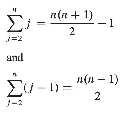
If the array is in reverse sorted order—that is, in decreasing order—the worst case results. We must compare each element A[j] with each element in the entire sorted subarray A[1 ... j - 1] and so tj = j for j = 2, 3, ..., n. Noting that
 we find that in the worst case, the running time of INSERTION-SORT is

We can express this worst-case running time as "an2 + bn + c" for constants a, b, and c that again depend on the statement costs ci; it is thus a quadratic function of n. Typically, as in insertion sort, the running time of an algorithm is fixed for a given input, although for some interesting “randomized” algorithms the running time can vary even for a fixed input.
Worst and average case analysis
We usually concentrate on finding only the worst-case running time, that is, the longest-running time for any input of size n.
- The worst-case running time of an algorithm gives us an upper bound on the running time for any input. Knowing it provides a guarantee that the algorithm will never take any longer.
- For some algorithms, the worst case occurs fairly often.
- The “average case” is often roughly as bad as the worst case.
The scope of average-case analysis is limited, because it may not be apparent what constitutes an “average” input for a particular problem. Often, it is assumed that all inputs of a given size are equally likely. Average case analysis is applied to the technique of probabilistic analysis.
Order of growth
We shall now make one more simplifying abstraction: it is the rate of growth, or order of growth, of the running time that really interests us. We, therefore, consider only the leading term of a formula (e.g., an2), since the lower-order terms are relatively insignificant for large values of n. We also ignore the leading term’s constant-coefficient, since constant factors are less significant than the rate of growth in determining computational efficiency for large inputs. For insertion sort, when we ignore the lower-order terms and the leading term’s constant-coefficient, we are left with the factor of n2 from the leading term. We write that insertion sort has a worst-case running time of θ(n2) (pronounced “theta of n-squared”).
We usually consider one algorithm to be more efficient than another if its worst-case running time has a lower order of growth. Due to constant factors and lower-order terms, an algorithm whose running time has a higher order of growth might take less time for small inputs than an algorithm whose running time has a lower order of growth. But for large enough inputs, a θ(n2) algorithm, for example, will run more quickly in the worst case than a θ(n3) algorithm.
References:
- Cormen, Thomas H, and Thomas H. Cormen. Introduction to Algorithms. Cambridge, Mass: MIT Press, 2001. Print.
