Insertion sort used the incremental approach to designing algorithms; having sorted the array A[1..j-1], we inserted the element A[j] in its correct position.

Now, we look at the divide and conquer approach to designing algorithms, post which we will use this approach to develop a sorting algorithm whose worst-case running time is much lesser than the insertion sort algorithm.

Divide and Conquer

Many algorithms use recursion to simplify the problem. What is recursion?

It is a technique in which a procedure or a function calls itself one or more times to solve closely related sub-problems.

The algorithms that use recursion typically follow a divide-and-conquer approach: they break the problem into several sub-problems similar to the original problem but smaller in size, solving the sub-problems recursively, and then combine these solutions to create a solution to the actual problem.

Steps:

1. Divide: Divide the problem into several sub-problems that are smaller instances of the same problem.
2. Conquer: Conquer the sub-problems by solving them recursively. If the sub-problem sizes are small enough, solve them directly.
3. Combine: Combine the solutions to the sub-problems into the solution for the original problem.

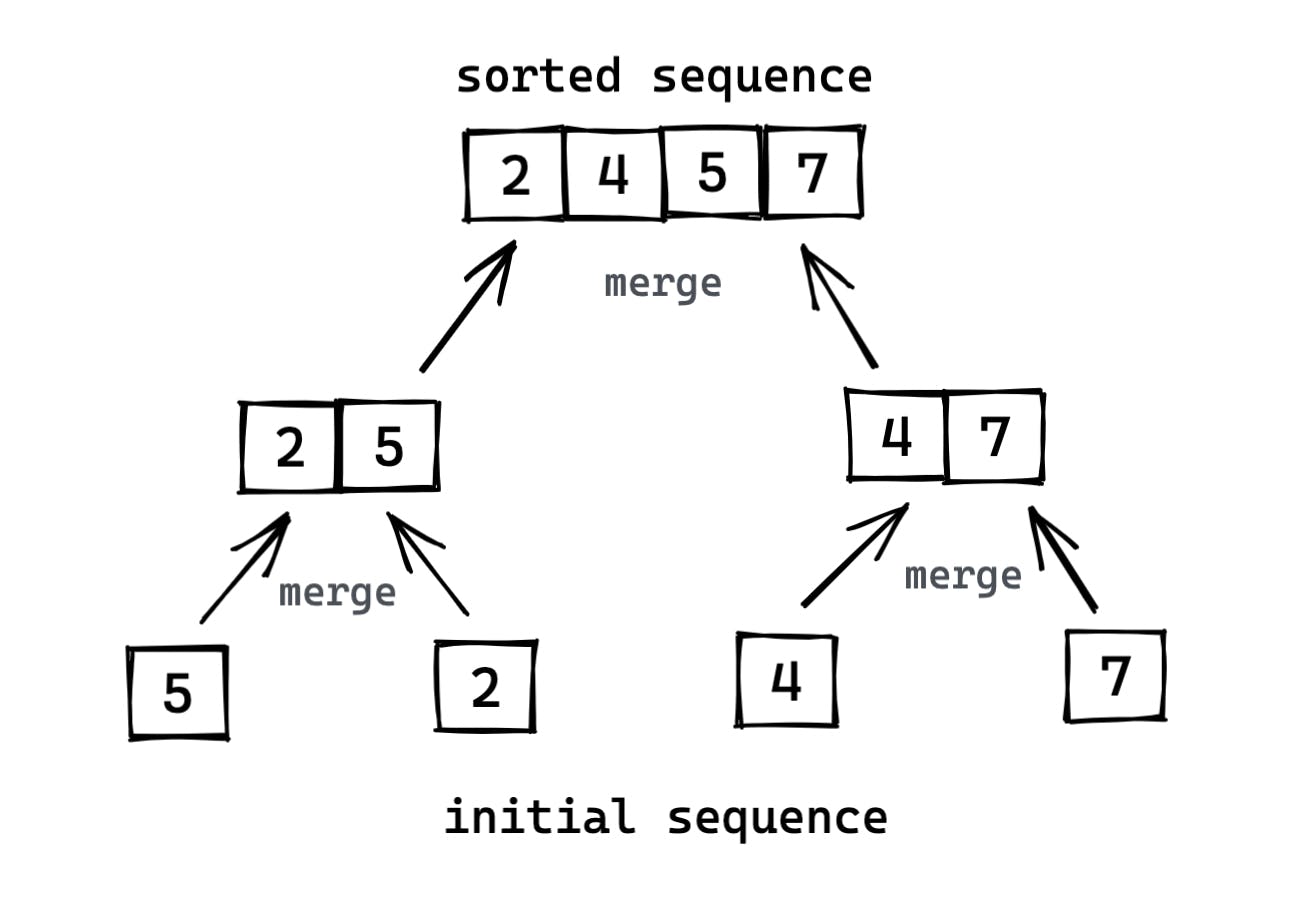
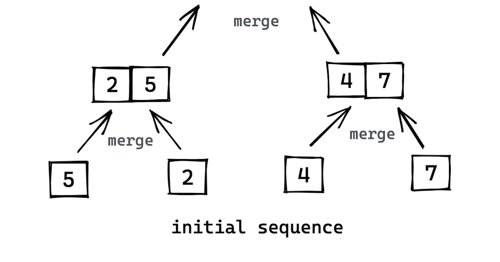
The merge sort algorithm follows the divide-and-conquer approach to solve the sorting problem:

1. Divide: Divide the sequence of n elements into subsequences of n/2 elements.
2. Conquer: Sort the subsequences of n/2 elements recursively, using merge sort.
3. Combine: Merge the sorted subsequences to form the final sorted sequence of size n.

The recursion "bottoms out" when the sequence to be sorted has the length 1 since every sequence of length 1 is already in sorted order.

The key operation of the merge sort algorithm is the merging of the two sorted arrays in the "combine" step. We merge by calling an auxiliary procedure MERGE(A, p, q, r), where A is an array and p, q, and r are indices into the array such that p <= q < r. The procedure assumes that A[p...q] and A[q + 1...r] are in sorted order and. It merges them to form a single sorted subarray that replaces the current subarray A[p...r].

MERGE(A, p, q, r)
1.  n1 = q - p + 1
2.  n2 = r - q
3.  let L[1...n1 + 1] and R[1...n2+1] be new arrays
4.  for i = 1 to n1
5.      L[i] = A[p + i - 1]
6.  for j = 1 to n2
7.      R[j] = A[q + j]
8.  L[n1 + 1] = ∞
9.  R[n2 + 1]  = ∞
10. i = 1
11. j = 1
12. for k = p to r
13.     if L[i] <= R[j]
14.         A[k] = L[i]
15.         i = i + 1
16.     else
17.         A[k] = R[j]
18.         j = j + 1

In detail:

• Line 1 & 2 - compute the length n1 and n2 of the subsequences A[p..q] and A[q + 1..r]
• Line 3 - Initialise arrays L and R ("left" and "right") of lengths n1 + 1 and n2 + 1. The extra position in each array will hold the sentinel.

  We use ∞ as the sentinel value so that we do not have to keep checking if we have reached the end of a subarray, since all values will be less than the sentinel value, other than ∞ in the other subarray of course. (sentinel - a soldier or guard whose job is to stand and keep watch.)

• Line 4-5 & 6-7 - copies the subarray A[p..q] into L[1..n1] and A[q + 1..r] into R[1..n2]
• Line 8 & 9 - Put the sentinels at the end of the arrays L and R
• Line 10 & 11 - Initialise indexing variables i & j
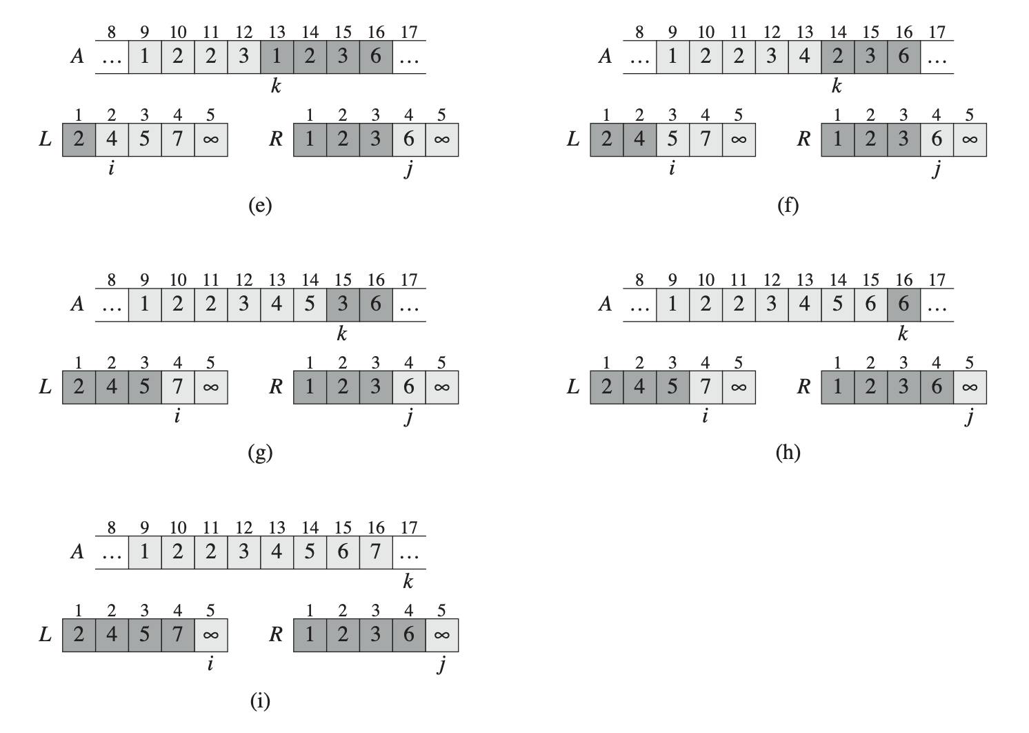
• The steps carried out in lines 12-18 are illustrated in the following figure with an example in the call MERGE(A, 9, 12, 16), when the subarray A[9..16] contains the sequence [2, 4, 5, 7, 1, 2, 3, 6]. After copying and inserting sentinels, the array L contains [2, 4, 5, 7, 1, ∞], and the array R contains [1, 2, 3, 6, 1, ∞].

The r + p - 1 basic steps are performed by maintaining the following loop invariant (defined in previous article, read here):
At the start of each iteration of the for loop of lines 12–18, the subarray A[p..k - 1] contains the k - p smallest elements of L[1..n1 + 1] and R[1..n2 + 1], in sorted order. Moreover, L[i] and R[j] are the smallest elements of their arrays that have not been copied back into A. (Prove that this loop invariant holds.)

The MERGE procedure runs in θ(n) time, where n = r - p + 1. Lines 1–3 and 8–11 take constant time. The "for" loops of lines 4–7 take θ(n1 + n2) = θ(n) time, and there are n iterations of the for loop of lines 12–18, each of which takes constant time.

Now, we use the MERGE procedure as a subroutine in the merge-sort algorithm.

MERGE-SORT(A, p, r)
1. if p < r
2.     q = ⌊(p + r) / 2⌋           // Note: floor of the value is taken
3.     MERGE-SORT(A, p, q)
4.     MERGE-SORT(A, q + 1, r)
5.     MERGE(A, p, q, r)

Analyzing divide-and-conquer algorithms

When an algorithm uses a recursive method to solve a problem, we can often describe its running time by a recurrence equation or recurrence, which describes the overall running time on a problem of size n in terms of the running time on smaller inputs. We can then use mathematical tools to solve the recurrence and provide bounds on the performance of the algorithm.

If the problem size is small enough, say n <= c for some constant c, the straightforward solution takes constant time, which we write as θ(1). Suppose that our division of the problem yields a subproblems, each of which is 1/b the size of the original. It takes time T(n/b) to solve one subproblem of size n/b, and so it takes time aT(n/b) to solve a of them. If we take D(n) time to divide the problem into subproblems and C(n) time to combine the solutions to the subproblems into the solution to the original problem, we get the recurrence:

Analysis of merge sort

For simplicity, we assume that the original problem size is a power of 2. Each divide step then yields two subsequences of size exactly n=2. This assumption does not affect the order of growth of the solution to the recurrence.

We reason as follows to set up the recurrence for T(n), the worst-case running time of merge sort on n numbers. Merge sort on just one element takes constant time. When we have n > 1 elements, we break down the running time as follows.

1. Divide: The divide step just computes the middle of the subarray, which takes constant time. Thus, D(n) = θ(1).
2. Conquer: We recursively solve two subproblems, each of size n=2, which contributes 2T(n/2) to the running time. (a = b = 2 for merge sort)
3. Combine: We have already noted that the MERGE procedure on an n-element subarray takes time θ(n), and so C(n) = θ(n).

Thus,

aT(n/b) + D(n) + C(n) = 2T(n/2) + θ(1) + θ(n) 
                      = 2T(n/2) + θ(n)     ..since, θ(1) + θ(n) = θ(n)

The recurrence for the worst-case running time T(n) of merge sort:

The "master theorem" (in a later article), can be used to show that T(n) is equal to θ(n*lg(n)). Because the logarithm function grows more slowly than any linear function, for large enough inputs, merge sort, with its θ(n*lg(n)) running time, outperforms insertion sort, whose running time is θ(n^2), in the worst case.

We use a recursion tree to find the value of T(n) here.

where the constant c represents the time required to solve problems of size 1 as well as the time per array element of the divide and combine steps.

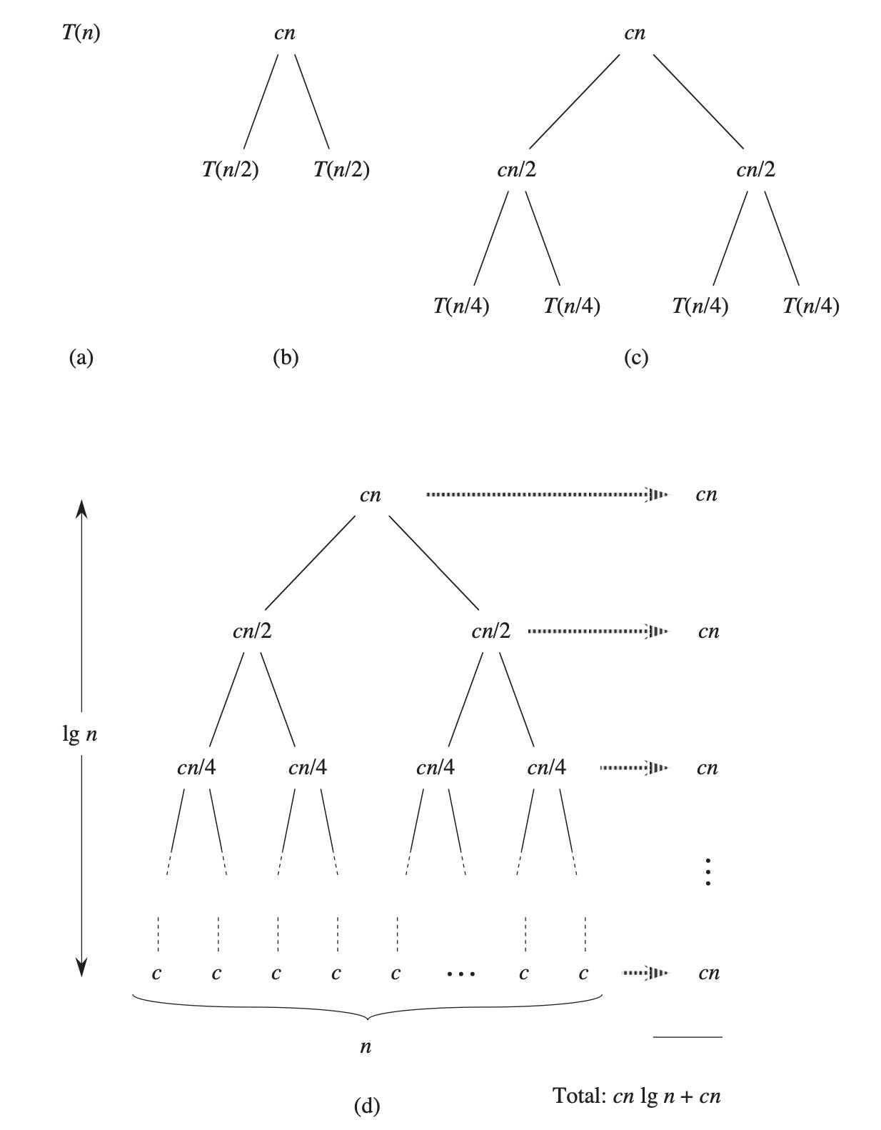
The following diagram of the recursion tree shows how we can solve the above recurrence. For convenience, we assume that n is an exact power of 2. Part (a) of the figure shows T(n), which we expand in part (b) into an equivalent tree representing the recurrence. The cn term is the root (the cost incurred at the top level of recursion), and the two subtrees of the root are the two smaller recurrences T(n/2). We continue expanding each node in the tree by breaking it into its constituent parts as determined by the recurrence until the problem sizes get down to 1, each with a cost of c. Part (d) shows the resulting recursion tree.

Next, we add the costs across each level of the tree. The top level has total cost cn, the next level down has total cost cn/2 + cn/2 = cn, the level after that has total cost cn/4 + cn/4 + cn/4 + cn/4 = cn, and so on. In general, the level i below the top has 2ⁱ nodes, each contributing a cost of c(n/2ⁱ), so that the ith level below the top has a total cost 2ⁱc(n/2ⁱ) = cn. The bottom level has n nodes, each contributing a cost of c, for a total cost of cn.

The total number of levels of the recursion tree is lg(n) + 1, where n is the number of leaves, corresponding to the input size. An informal inductive argument justifies this claim.

The base case occurs when n = 1, in which case the tree has only one level. Since lg(1) = 0, we have that lg(n) + 1 gives the correct number of levels. Now assume as an inductive hypothesis that the number of levels of a recursion tree with 2ⁱ leaves is lg(2ⁱ) + 1 = i + 1 (since for any value of i, we have that lg(2ⁱ) = i). Because we are assuming that the input size is a power of 2, the next input size to consider is 2^{i + 1}. A tree with n = 2^{i + 1} leaves has one more level than a tree with 2ⁱ leaves, and so the total number of levels is (i + 1) + 1 = lg(2^{i + 1}) + 1.

To compute the total cost represented by the recurrence, we simply add up the costs of all the levels. The recursion tree has lg(n) + 1 levels, each costing cn, for a total cost of cn(lg(n) + 1) = cn*lg(n) + cn. Ignoring the low-order term and the constant c gives the desired result of θ(n*lg(n)).